Overview

This project converts an analogue signal and displays its frequency components in the form of a spectrum of 7 octave bands on an OLED display. To do this, it uses a Fast Fourier Transform (FFT) which is a sampling theorem that is a fundamental bridge between continuous-time signals (analogue signals) and discrete-time signals. It uses a sample rate that enables discrete sequences of samples to capture all the information from a continuous-time signal of finite bandwidth.

Two versions are supported, an ESP8266 variant that can analyse analogue signals with a maximum frequency of 5100Hz (5.1 KHz) using a sample size of 256 elements. This limit is determined by the Analogue to Digital Converter (ADC) speed which can convert at a rate of approximately 10 KHz. The second is an ESP32 variant that can analyse analogue signals with a maximum fundamental frequency of 20,000Hz (20.0 KHz) with a sample size of 512 elements. This limit is determined by the Analogue to Digital Converter (ADC) speed which can convert at a rate of approximately 40 KHz.

The system is comprised of the processor either ESP8266 or ESP32, an OLED display either 0.96″ or 1.3″ and a audio microphone unit that is comprised of an electret microphone and amplifier. The received audio is applied to the ADC input of the process.  Note: Most ESP8266 development boards have an on-board voltage divider to limit input voltage, for example on the WEMOS D1 Mini 5v peak-peak are reduced to 1v peak-peak. The ESP32 tends not to have any input voltage dividers.

FFT Elements – Sample Size and Sampling frequency

Sample Size – The FFT-algorithm defines a set of samples for the analysis results to be stored in. For most algorithms, the number of samples is usually a factor of 2, so 16, 32, 64, 128 or 256 are not unusual. The greater the number of samples the more time it takes to convert an analogue signal, but the greater the frequency resolution and discrimination will be.

Sampling Frequency – Reference to the Nyquist-Shannon Sampling Theorem says sampling of an analogue signal needs to be at least twice the frequency of the signal being analysed, this limits the maximum frequency to half of the sampling frequency.

FFT Visualisation – From a time domain Waveform to Frequency Domain

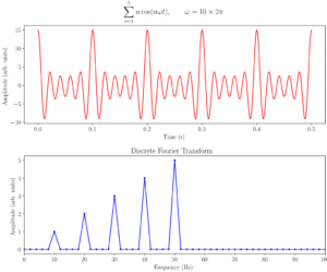
The diagram above illustrates a square wave (coloured red) in the time domain, which refers to a view of the waveform with respect to amplitude and time, it therefore shows how the waveform changes over time.

This is then overlaid with a frequency domain plot showing a representation of the individual frequency components and their phase relationships that form together to create the example square wave.

In a Fourier transform analysis converts the function’s time-domain representation, shown in red, to the function’s frequency-domain representation, shown in blue. The component frequencies and amplitudes are spread across the frequency spectrum chosen for analysis and are represented as peaks in the frequency domain.

In this code example, the Fast Fourier Transform (FFT) is used, which is an algorithm that computes discrete Fourier transforms of the sampled waveform thereby enabling the waveform to be changed from its original time domain to the frequency domain. The FFT rapidly computes such transformations by factorising the result into a matrix/array. In the code the result arrays of real and imaginary components are called:

double vReal[SAMPLES];

double vImag[SAMPLES];

In the array vReal and vImag this contains what is called the complex number results separated into the mathematical parlance of Real (vReal) and Imaginary (vImag) components.

Modulus and argument

The contents of the arrays vReal and vImag contain the coordinates in the complex number in whats called polar coordinates that refers to the distance of a point (diagram above refers) of origin z from the origin (O), and the angle subtended between the positive real axis (Re) and the line segment Oz in a counter-clockwise sense. This leads to the polar form of complex numbers.

The absolute value (or modulus or magnitude) of a complex number is defined as z = x + jy where ‘j’ is an imaginary operator.

Its amplitude is derived from z = sqrt(a² + b²)

In the code once the sampling of a waveform has been completed and the result captured in the array elements of vReal[] noting we can ignore the phase angle for the analysis so vImag[ ] array elements are always assigned to 0.

Next the array vReal is analysed by the FFT function, as follows:

FFT.Windowing(vReal, SAMPLES, FFT_WIN_TYP_HAMMING, FFT_FORWARD);

Then:

FFT.Compute(vReal, vImag, SAMPLES, FFT_FORWARD);

Then:

FFT.ComplexToMagnitude(vReal, vImag, SAMPLES);

Understanding the results

Now after the analysis, the array vReal[] contains the amplitude of each frequency component where the index of the array  ‘I’ represents the pointer to the amplitude of each frequency component, thus:

i = 0                        : The DC component

i = 2                        : Fundamental frequency e.g. 1000 Hz

i = n onwards     : Each value of ‘i’ provides the amplitude of the frequency component

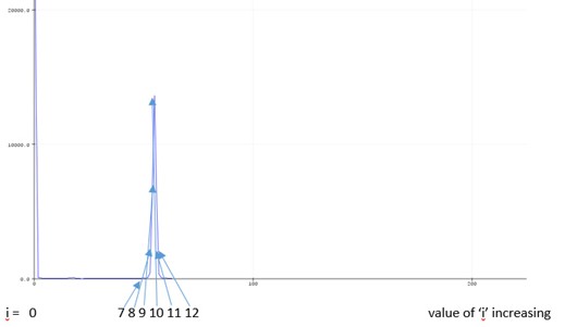
In this example you can see that as the index ‘i’ increases the magnitude in the array vReal also increases, this gives the characteristic growth in amplitude of the frequency amplitude, it shows that at i = 7 the value is zero, then at 8 and 9 the amplitude is starting to climb then at 10 it reaches a peak then at 11 it is down to zero again. This repeats across the whole frequency spectrum.